
Anonymization is a hot topic of discussion. We are generating and collecting huge amounts of data, more than ever before. A lot of this data is personal and needs to be handled sensitively. In recent times, we’ve also seen the introduction of the GDPR stipulating that only anonymized data may be used extensively and without privacy restrictions.
For a number of years, we have been working with anonymization using KNIME. In this blog we would like to share the nodes we’ve developed with the community. These nodes help address privacy requirements. For the purposes of this article, we assume you are familiar with various anonymization techniques and terms. Our walkthrough of the Privacy extension is based on and example workflow.
Why are these anonymization nodes important? Lack of proper anonymization or pseudonymization introduces risks and, if there is a data breach, huge penalties are applied for non-GDPR compliance. Even if you think you have analyzed your data and believe it to be anonymized, our assessment node can measure the risks. Simple anonymization is not enough.
Goals of this article
- Demonstrate how to work with the Redifled Privacy Nodes for KNIME, which utilizes advanced anonymization techniques
- Provide concrete examples of personal data anonymization and assess the risks de-anonymization
Dataset
The reference data we use is from the computer game FIFA 19. It contains “personal” data about real football players – their names, physical parameters, ages, salaries, clubs, positions and some in-game parameters.
Introducing the Redfield Privacy Nodes
Our Privacy Extension contains three different node types, which handle these areas: basic anonymization, hierarchical anonymization, and assessment node.
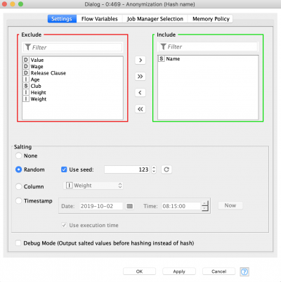
- Anonymization node – applies hashing (SHA-1) with salting to the selected columns. There are four salting modes:
- None: the selected values are hashed as they are, no additional concatenation is used
- Random: random seed is used for salting every time node is executed. A fixed seed value can be used
- Column: values from additional columns are used for salting. Values from selected columns are concatenated row-wise
- Timestamp: the selected date and time is used for salting. Selected Date&Time is concatenated to the values. It is possible to use workflow execution time.
- Hierarchical nodes apply a technique to generalize the quasi-identifying attributes. These nodes utilize a powerful anonymization Java library, called ARX.
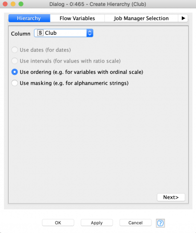
- Create Hierarchy node: builds the hierarchies used in the Anonymization node. There are four types of hierarchies, their selection depends on the data type of the attribute and the way the user would like to anonymize the data: date-based, interval-based, order-based and masking-based
- Hierarchy Reader node: has two functions – reads the binary file of hierarchy and/or updates the hierarchy to fit the input dataset
- Hierarchy Writer node: writes the created or updated hierarchies to the disk as binary files
- Hierarchical Anonymization node: applies the hierarchy input, utilizes the capabilities of ARX library, and anonymizes data according to five currently available models. In most cases, hierarchy files are necessary for anonymization. These files can be fed to a special ARX Hierarchy Anonymization port or could be read by the node
- Anonymity Assessment node: estimates two type re-identification of risks: quasi-identifiers diversity and attacker models.
- The first type of risk assessment includes calculation of distinction and separation metrics for the quasi-identifying attributes.
- The second type of risk assessment estimates three classical types of attacks (http://dx.doi.org/10.6028/NIST.IR.8053): the prosecutor, the journalist and the marketer.
The output table contains the probabilities of re-identifying the records in the input table. This node has second optional input port, that allows the user to compare data before and after anonymization.
You can read more about ARX capabilities in one of the papers of the creator of the library Dr. Fabian Prasser.
Concept behind anonymization methods
To better understand this article and our example workflow you need to know some of the concepts behind the methods used for anonymization.
Attribute types
ARX defines four attribute types and we apply the same definitions:
- Identifying attributes identify a person precisely, e.g. name, surname, address, social security number.
- Quasi-identifying attributes identify a person in a dataset indirectly e.g.the attacker could identify a person if additional information is available in the dataset, e.g. age, date of birth, gender, zip code.
- Sensitive attributes contain information that is not referred to identifying, however it will be exposed, and should not be able to be matched to a specific person, e.g. medical diagnoses, sexual orientation, religious views.
- Non-sensitive attributes do not refer to any of the types described above, but can be useful for data analysis.
Forms of data transformation
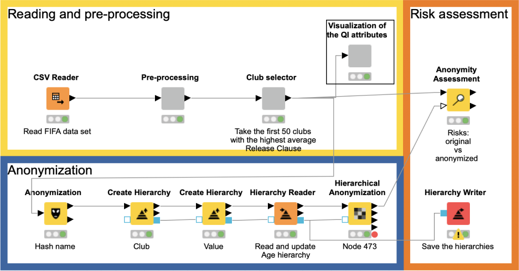
In the following example we are going to utilize our Privacy Extension for data anonymization. To do so, we have to build two hierarchies that are necessary for hierarchical anonymization methods provided by ARX. We will read and update the hierarchies that were created before to make them fit the current dataset, save all the used hierarchies, and finally compare the risks of de-anonymization for the original and the anonymized dataset.
The idea behind data anonymization is to: transform the data such that afterwards it will be impossible or hard to re-identify the persons who present in the dataset. There are many ways to transform data and hide information, however in this extension we use these four:
- Suppression – entire removal of values in specific columns. Usually used for deleting identifying information – name, surname, address.
- Character masking – partial modification of values with non-meaningful characters (e.g. “x” or “*”). Can be applied to hide quasi-identifying attributes – zip code, IP, phone number.
- Pseudoanonymization – replacement of values with values that do not contain any useful information. The simplest examples of this are hashing and tokenization. Pseudoanonymized data can be reversed if the reversal algorithm is known or translation table is stored. This type of transformation can be applied to almost any kind of attribute.
- Generalization – reduction of the data quality by providing some aggregated data instead of original values. Applying functions like mean, median, mode or binning the data are examples of data generalization.
Data anonymization models
Data anonymization models are based on the many models available for this in the ARX library. The choice of model depends on multiple factors: sensitive attributes present in the dataset, types of attacks to prevent, size and diversity of the dataset, etc. Our Redfielfd Privacy Nodes extension has five models – this list will be extended in future releases.
Let’s now have a look at the simplest model – k-anonymity defined as follows: “A dataset is k-anonymous if each record cannot be distinguished from at least k-1 other records regarding the quasi-identifiers. Each group of indistinguishable records in terms of quasi-identifiers forms a so-called equivalence class.”
Risk assessment
The extension includes two risk assessment approaches: quasi-identifiers risks and attacker model risks.
The quasi-identifiers approach is based on calculation of distinction and separation of the quasi-identifiers and their combinations to find out which attributes have the biggest diversity. Separation defines the degree to which combinations of variables separate the records from each other and distinction defines to which degree the variables make records distinct.
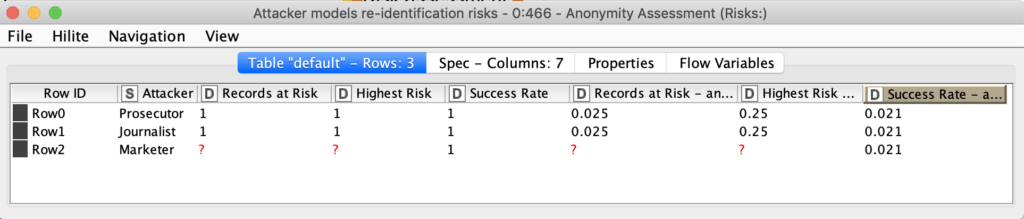
The attacker model assesses the risk of an attack. There are three attacker types. This approach estimates the probability of re-identification and success rate for each of them.
- Prosecutor: tries to identify a specific person in the dataset.
- Journalist: tries to identify any person in the dataset, to show that the dataset is compromised.
- Marketer: tries to identify as many people in the data set as possible.
For additional details on risk analysis refer to ARX web site.
Football stars and the example workflow
Now let’s get back to the FIFA19 dataset we said we’d use in our example workflow. Our aim is that the output from the workflow will provide a dataset that cannot re-identify any of the players. A risk assessment is performed to make sure that the players cannot be re-identified based on the two approaches, quasi-identifier attributes and risks of attacks.
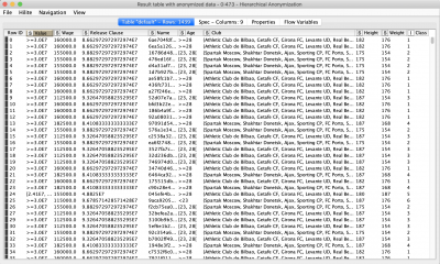
The FIFA19 data set contains 88 columns. We will reduce this number for simplicity’s sake. In the “Pre-processing” component we filter the columns to leave only: Name, Age, Club, Value, Wage, Height, Weight, Release Clause. The next step involves conversion from strings to numbers and deleting rows with missing values.
In the next component we select the clubs with the highest average Release Clause. This component has a Configuration node inside enabling the user to choose how many clubs should be taken into consideration (the default is 50). Next, the Visualization component creates three distribution plots of the quasi-identifying attributes, which we will anonymize later. It is good practice to visualize the data with histograms, bar charts and sunburst diagrams in order to understand how homogeneous your data is: are there any potential clusters or outliers, for example? This is extremely helpful for building the anonymization hierarchy.
Anonymization node
The Anonymization node is the first one we’ll use to anonymize the names of the football players. It utilizes simple technique – hashing; but we can also apply salting (here: fixed seed) to make the anonymization more secure. An added benefit of this approach is that it enables you to get back to the original data since the translation table is available at the second output port.
Once we have hashed the identifying attributes, we can move on to more sophisticated anonymization methods.
Building hierarchies
The idea of building a hierarchy is to define complex binning rules with multiple layers that go from original data (i.e. the unmodified data) to less and less accurate, and finally to completely suppressed data. There are four types of hierarchies in ARX:
- Interval-based hierarchies: for variables with a ratio scale.
- Order-based hierarchies: for variables with an ordinal scale.
- Masking-based hierarchies: this general-purpose mechanism allows creating hierarchies for a broad spectrum of attributes, by simply replacing the characters with “*”.
- Date-based hierarchies: for time series data.
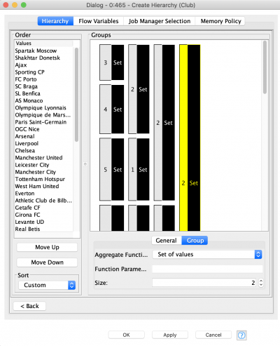
In this walkthrough, we will also restrict the number of used hierarchies and use only the first two types. An order-based hierarchy is used when generalizing categorical data. We are going to use it to generalize the clubs (figure 3). First, we need to order the clubs manually: at first we take the three outlier clubs which are the only representatives of their country, then four Portuguese clubs, then bigger sets of French, English, Spanish, German and Italian clubs. At the first level of the hierarchy we merge the clubs by country, at the second level we are merging outliers with Portuguese clubs and German clubs with Italian ones. At the higher levels we continue merging the clubs more and more. At the final layer of the hierarchy the information will be completely suppressed (all values will be replaced by “*”) by default. In order to define the size of the set, click a group and define its size. To add the next hierarchy level right click it and click “Add New Level”, then define the size of the next level and so on.
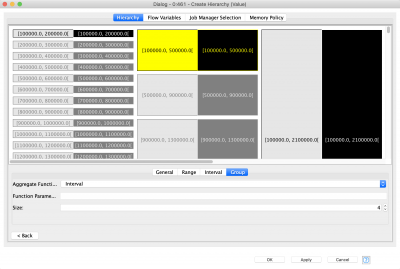
Preparing the interval-based hierarchy is a bit more complicated. First you need to define the general range of the number within which more detailed ranging will be performed . Do this by clicking the “Range” tab and setting up the values for “Bottom coding from” and “Top coding from”. For simplicity we are going to set up the same values as snap values for both the upper and lower bounds. Snap settings are used in case values fall into an interval stretching from the bottom coding or top coding limit to the “snap” limit, it will be extended to the bottom or top coding limit. All values outside the general interval will always be considered outliers and are put into two special bins: more than higher limit and less than lower limit.
Now you have to double-click the only interval that is available at the beginning, and set up Min and Max values for it. This will be the smallest bin size. Adding other levels of interval-based hierarchy is similar to the previous example – add the level and define its size.
Next node that we are going to use is “Read Hierarchy” – this node is used for reading hierarchy files that were created before and update them according to the current dataset. This is a requirement of ARX algorithms: even if a new dataset has the same structure (column names and data types) it can still have different ranges of values, which is why it should be updated.
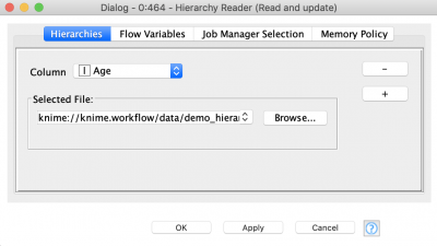
The settings of the node are pretty straightforward – select the column that is going to be fetched by hierarchy and provide a path to a hierarchy file. The node is capable of reading multiple hierarchies at a time.
Hierarchical anonymization
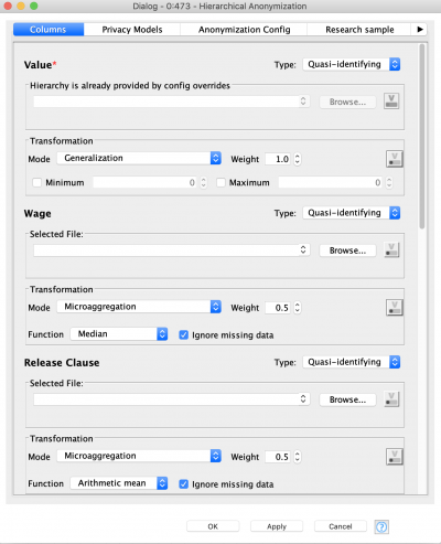
Now let’s finally apply Hierarchical Anonymization. To do this we need to feed the node data table and hierarchy configuration. At the first “Columns” tab you need to specify the attribute types. By default they are always identifiers. Once you change the attribute to quasi-identifying the dialog window automatically changes and asks you for more settings.
The most important are hierarchy, mode, and weight. If hierarchy is already provided (via blue port) the attribute will be marked by a red asterisk to the right of its name. It is also possible to provide a path to the hierarchy file.
There are three modes available for data anonymization: generalization, microaggregation and clustering, and microaggregation. The default mode is generalization and hierarchy is only required for it, however for some attributes we are going to use microaggregation. For the latter mode it is necessary to select the aggregation function.
The weights define the importance of the attributes, which means that the algorithm will try to suppress and generalize the attributes less with higher weights. Default values for every quasi-identifying attribute is 0.5.
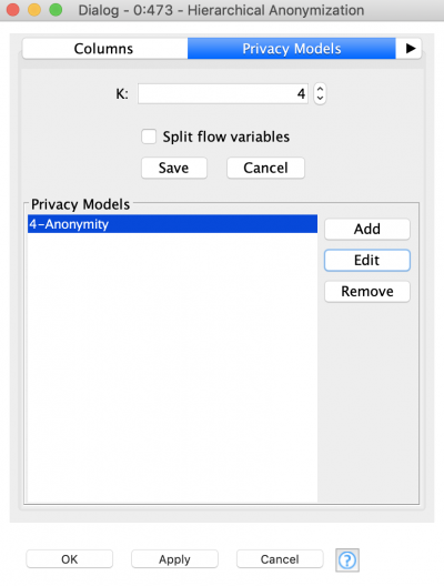
Once all attributes types are defined, and the modes and weights set up, it is time to select an anonymization model. Do that by switching to the next tab – “Privacy Models”. As we said before, we want to use k-anonymity model, with k=4. Basically it means that after anonymization, the highest probability of re-identification of any record will be 1/k=¼=25%. It is also possible to use several different types of models at a time.
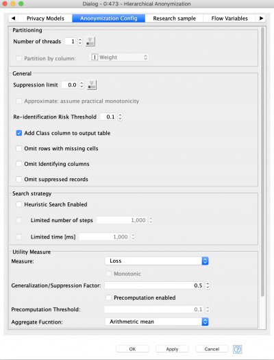
The next tab called “Anonymization Configuration” contains general settings, let’s go through some of them.
- Partitioning – this option allows us to split the dataset into several partitions. Each dataset is then anonymized independently using the same settings as a new thread. “Partitioning by column” means you split the dataset by the values of the column (e.g. gender, family status) After that all results will be concatenated into one. Users should be careful with this mode as although it can increase anonymization performance, the final result might not satisfy the requirements of the anonymization model. It is better to use it only when you are going to apply the same anonymization settings to different subsets, and you have some columns to distinguish them, for example by gender.
- Suppression limit – defines the ratio of records that can be completely suppressed during anonymization.
- Add Class column to output table – if active adds a column with a number of equivalence class of every record.
- Omit Identifying columns – after anonymization, columns marked as identifying area excluded from the result table.
- Omit suppressed records – if any records (rows) were completely suppressed they will have only “*” for every quasi-identifying attribute – these records are excluded from the result table.
- Heuristic Search Enabled – this is a stop criteria for an algorithm that is defined by the number of iterations or amount of time spent before algorithm stops.
- Generalization/Suppression Factor – a value that defines the preference during data transformation: 0 stands for generalization, 1 for suppression.
Risk assessment
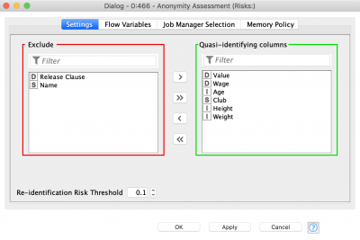
The next node in the workflow is Anonymity Assessment. It has two input ports, one of them is optional so it possible to not just assess the risks, but also compare them for original and anonymized datasets.
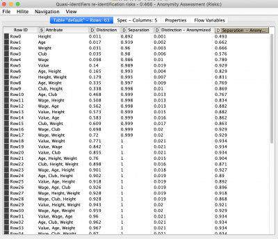
As we can see the distinction and separation values decreased after anonymization. This table provides insight into the attribute’s significance in terms of person identification. We can also assess how combinations of different quasi-identifying attributes might lead to person re-identification.
The second table returns the results of risk assessment for three types of attacker models. The most interesting column is “Records at Risk”, showing the percentage of records at risk of being re-identified as per the threshold value. We used the default threshold value – 0.1. After anonymization we can see, that only 0.025 records exceed this risk. A pretty good result.
Conclusion
In this blog post we presented an overview of the Redfield Privacy Nodes extension for KNIME which uses different algorithms for anonymization and the assessment of re-identification risks. We implemented hashing with salting technique for reversible anonymization. Then a sophisticated hierarchical anonymization was applied. And finally we assessed the risks before and after anonymization.
The core technology for the hierarchical anonymization and assessment is based on powerful ARX Java library. ARX is also available as a desktop app – please check it out https://arx.deidentifier.org/downloads/.
We debated over the length of the blog post and if it should be split into multiple blog posts since there is a lot to absorb. But we think it is important to give a full picture and explain all the tools belonging to the privacy nodes. We would love to hear from you what parts of the blog you would like to hear more about in our future articles. Feel free to contact us. And also check our previous blog post Will They Blend: KNIME Meets OrientDB, about KNIME and OrientDB integration.
How to install the Redfield Privacy Nodes
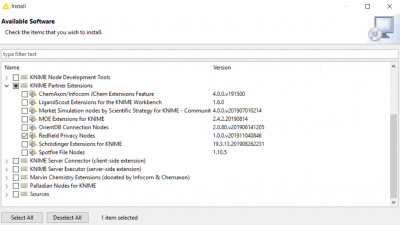
Go to File -> Install KNIME Extensions
From the list, expand the KNIME Partner Extensions and select “Redfield Privacy Nodes”.
About Redfield:
Redfield is fully focused on providing advanced analytics and business intelligence since 2003. We implement the KNIME analytics platform for our clients and provide training, planning, development, and guidance within this framework. Our technical expertise, advanced processes, and strong commitment enable our customers to achieve acute data-driven insights via superior business intelligence, machine and deep learning. We are based in Stockholm, Sweden.