It has been 2 years since we have released our nodes to connect graph database Neo4j with data analysis tool Knime. Now it is about time to update and get rid of the (known) bugs. In the latest update the major thing that we have developed is the batch mode, that increases the performance of the Cypher queries significantly. And also it is very convenient now, as long as you prepare the batch query with just a couple of clicks.

Today we are going to demonstrate both how to use the batch mode and how to use Neo4j native Graph Data Science (GDS) library that will help you enrich your capabilities of Knime.

The use case

We are going to work with a data set that represents the social network of group members and the interest groups (based on Kaggle data set). The idea is to train a model that will classify members as influencers and non-influencers based on their graph embeddings. This way we will read this information from CSV files and then push the data to Neo4j using batch mode, then we will do feature engineering with GDS, then extract features from graph and train two models in Knime. We will also plot the graph embeddings with the help of t-SNE. The workflow is available on Knime Hub.

Data preparation

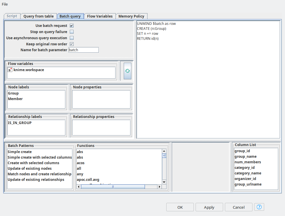
The data preparation will not take that long, since the data is already presented in a good shape, the only thing we have to do is to get rid of some missing values from the members data set. Then we can directly jump to ETL with batch mode. First we need to add an optional table input port to feed in the table with group information. Then in the dialog (see figure 1) we need to activate “Use batch request” mode and switch to the “Batch query” tab. This tab looks very similar to the “Script” tab where a user can define a single query. However here we have the same as for “Script” features: the list of nodes and relationships with their properties, list of function, flow variables. But also we have some extra features: list of column of input table and list of batch queries examples. Everything can be added to a query body with just a double-click. The query examples will help to immediately get the syntax of the batch queries, so you can just paste them in, and start adjusting according to your data and graph schema. In the batch query we refer to a variable with the name “batch” by default, it keeps the input data, but you can always rename it if you wish. Then the input data is unwinded and you can use it along with standard operations such as CREATE, MATCH and MERGE. Now it becomes so easy to map the input table data into the property values of nodes and relationships. Then the node will automatically generate multiple batch scripts according to the provided pattern. The performance of this operation is way faster than running the single queries even using asynchronous mode.

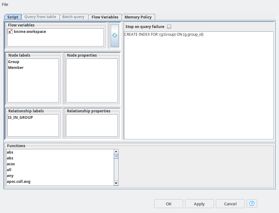
So once groups are in place, we need to do a similar upload for Members. In order to increase the MATCH queries performance we create the indices for group_id and member_id using Neo4j Writer node with “Script” mode.

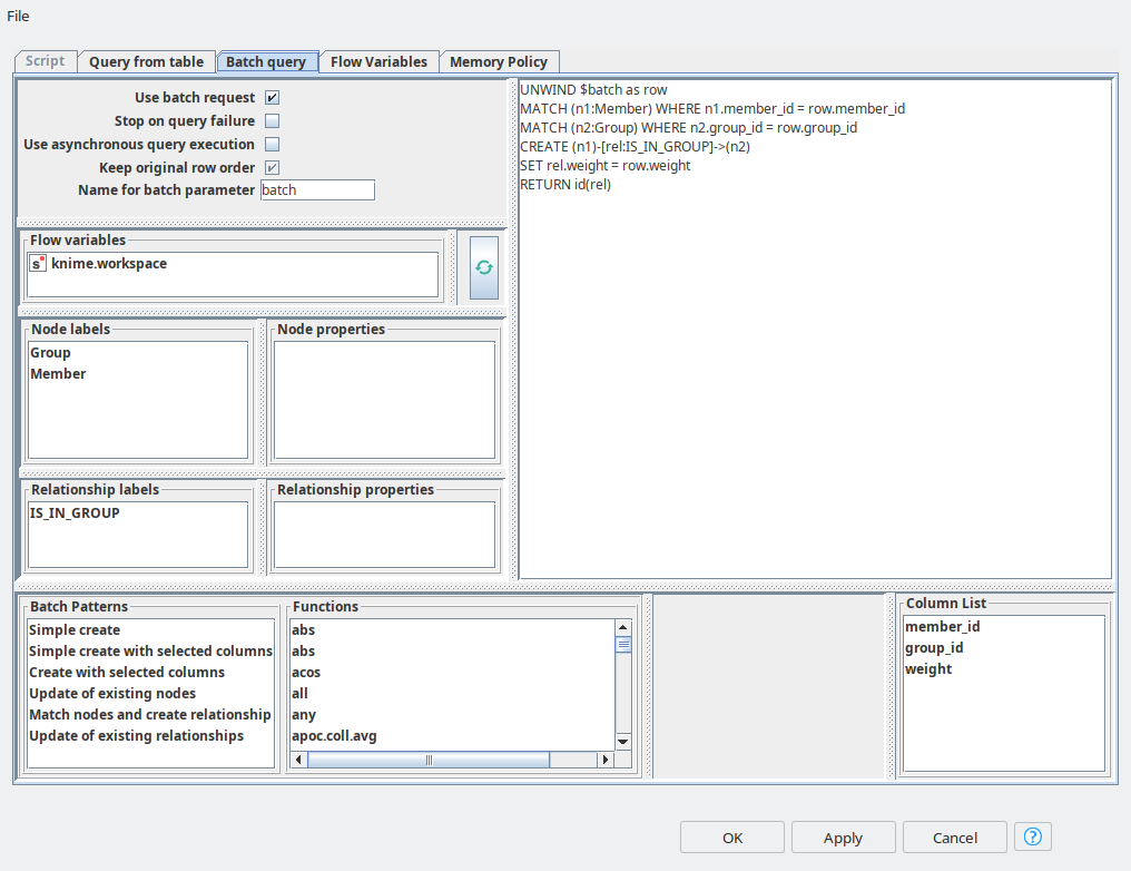
And the final step in data import is to create relationships between Member and Group entities. For this purpose again we are using Neo4j Writer node with “Batch query” mode, and here we can refer to the pattern called “Match nodes and create relationships”. We just need to paste in the right properties for matching – group_id and member_id. And the relationship between the nodes has weight, so we set it up as a property.

Feature engineering and preparing for ML

Once the data is in the graph we can start feature engineering. Neo4j already provides a powerful Graph Data Science library that has a set of many graph-related algorithms. So, first of all to start applying GDS algorithms we need to create a memory graph with gds.graph.create. 

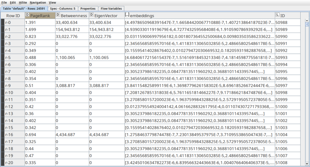
At the next step we are going to use the following algorithms to calculate graph metrics: PageRank, Betweenness centrality and Eigenvector centrality. These metrics will be useful for automatic labeling the data set for influencer and non-influencer members. Another GDS algorithm that we are going to use is SAGE – the neural network model that produces embeddings or vector representation of the graph. The main parameters here are the embedding dimension, the number of epochs for training the neural network and the features. As the features we are going to use the same graph metrics from the previous step. Note that for all the algorithms mentioned here we use mutate mode, so the embeddings and metrics are written to the node properties, so we do not have to calculate them every time and they can easily be extracted. These are all the features we need now. The final step here is to use the Neo4j Reader node to extract this data from the graph and import it to the Knime table.

Then we can start using graph metric algorithms to automatically label the members.To do so we will define an influencer by the following criteria:

• influencer has more connections with different groups;
• influencer use has more connection with the groups of similar kind (Sports, Cooking, etc);
• influencer is more devoted to the group, (let’s say participates in the most events, has more posts, etc), and we can estimate this devotion as a weight of the relationship between the Member and the Group.

As long as the graph metrics represent different types of significance of the node with the graph, and usually are based on the number of paths the node is part of, we can consider higher values of these metrics as a sign of influencer members. This way in the component called “Labeling members” we take the top 15% (85-percentile) of members that have the highest values and assign them to the influencers. The rest are assigned to be non-influencers.

ML, visualization and results

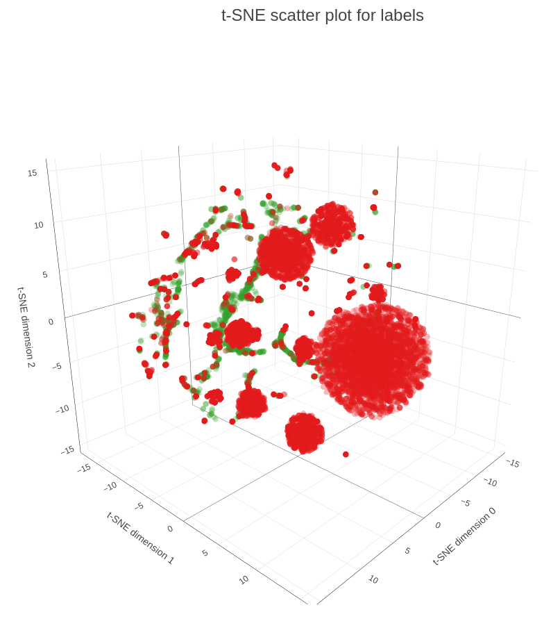
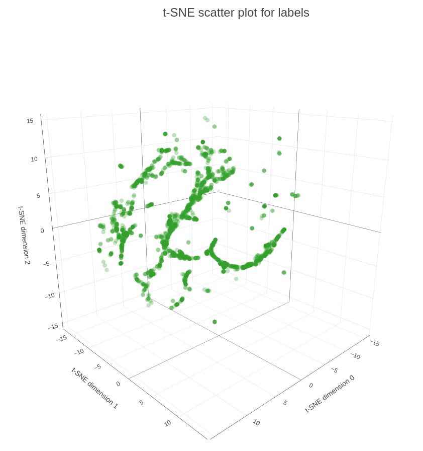
In the final part of our demo we are applying t-SNE procedure to map 32-embeddings to 3-dimensional space, so we can plot them on a scatter plot (see Figure 5). As you can see on the plot many of the influencers are scattered, meaning that they have diverse interests and are connected to multiple groups. At the same time we have influencers within the dense spheres that represent another type, so-called dedicated influencers, so they are connected to the groups of the same type and/or have higher weight. 

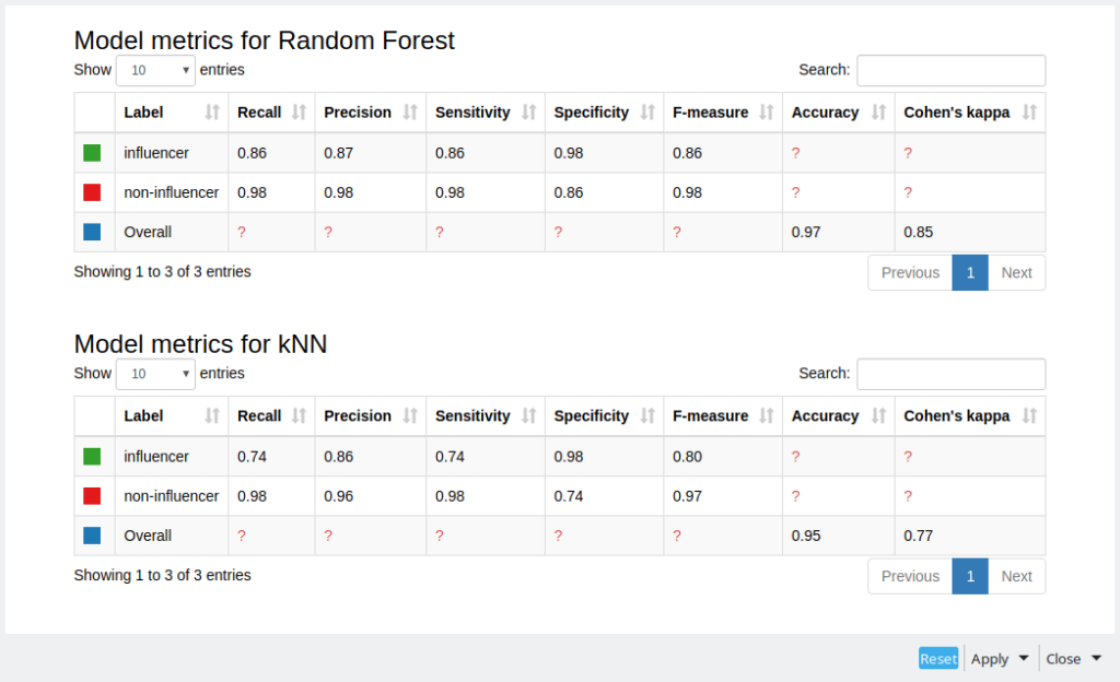
With the Partitioning node we are splitting the data to training and test data sets as we are going to apply supervised machine learning algorithms: random forest and k-nearest neighbors. Then finally we can estimate the predictive quality using Scorer nodes. As we can see from figure 6 Random Forest did slightly better based on F-measure for every class and overall Cohen’s kappa. Still the results are quite good, considering that we did not do any parameter optimization and we had an unbalanced data set.

As long as we already have a SAGE model, every time we update the graph with new data we can easily recalculate metrics and embeddings to get new predictions. Another approach that can be useful is to use metric learning in order to analyze the similarity between different types of members, moreover we go beyond just these 2 classes that we used and introduce more categories like the member group preferences using the same embeddings. The last approach might be very helpful for building a recommendation engine for members to join new groups.

But these ideas are beyond the scope of the current article, as the main purpose was to demonstrate how to work with batch queries using the Redfield Neo4j extension and how to combine the power of GDS and Knime.

Please note that the visualizations and model metrics in the paper and ones you will obtain after running the workflow might differ slightly due to stochastic distribution of initial parameters in SAGE, t-SNE, Random Forest and kNN.