- What is Topic Modeling?
- The Data Set
- Scraping the Data
- Preprocessing Data with Spacy to Do Topic Modeling
- Topic Modeling and Clustering
- Visualization and Analysis
- Conclusion
The Netflix platform generates a LOT of data daily! In this article, we will use data set from the Breaking Bad series and deep dive into our brand new solution, and do a topic modeling workflow to automatically assign labels to the series episode names.
Text processing or Natural Language Processing (NLP) is a big part of machine learning. The growing demand from the business perspective for NLP tasks, including topic modeling is outstanding in the current years.
The type of tasks to solve business problems can vary. Starting with the classical NLP techniques such as part of speech (POS) tagging, named entity recognition (NER), morphology analysis, and lemmatization. Moving up to more advanced techniques like text classification, similarity search, question answering, and text generation.
We have developed an extension for KNIME that includes the power of multiple algorithms acknowledged by the NLP community. Our extensions can be easily integrated with Spacy and BERT-based models within KNIME.
In this article, we are going to present a quite common approach – topic modeling. This approach can be applied for analyzing the feedback from customers or even your competitors. In the later case scraping techniques will be of use. This way our example will contain both scraping using Selenium Nodes and text processing using the Redfield NLP Nodes.
What is Topic Modeling?
Before deep diving into our use case, we want to cover the basics here.
Topic modeling is a part of text mining that helps to automatically find topics in the text and identify patterns hidden in it. With all data derived from the text, it is easier for a user to interpret the results and make a decision. Unlike rule-based text mining techniques, topic modeling does not use regular expressions and extracts sets of words typical for a specific text. These repeating bunches of words are called “topics” and they are specific for different fields.
The field of application of topic modeling is wide:
- processing large volumes of textual data
- extracting information from unstructured text
- clustering of documents
- feature selection
Most often topic modeling is used for:
- Social media monitoring when you need to know what’s trending on social media.
- In email/ticket filtering you can sort out different types of inquiries or set up your own spam filters.
- Dialog systems (chatbots) for better understanding of customer’s inquiries and auto responding which saves time for customer service department
- In hiring and recruitment keyword searches will identify relevant job applications.
Topic modeling comes in hand when big data sets need to be analyzed. Data set is a collection of related to the same topic pieces of data: schemas, points, tables, or (speaking of machine learning) objects that are understandable for machines so they can analyze them and make predictions. Search terms in Google, website statistics, customer reviews, marketing KPIs, weekly schedule – all these are examples of a data set.
And with no further due let’s dive into our data set that we will do topic modeling for.
The Data Set
The data we are going to scrape are the subtitles of the popular TV series Breaking Bad using the Selenium Nodes. The TV series includes 5 seasons, 10-15 episodes each, we are only going to analyze the text of the subtitles of dialogues for each episode. Then standard preprocessing methods like POS and NER tagging, stop words filtering, and lemmatization are applied to prepare the data for topic modeling with Latent Dirichlet allocation (LDA). And the final part of the blog post is dedicated to data analysis and visualization: here we are going to convert the documents to the vectors (document embeddings) and apply clustering and compare the topics and clusters, also we are going to create a tag cloud for the whole set of subtitles and finally, we are going to create a simple knowledge graph.
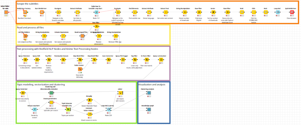
Figure 1. Workflow overview [you’ll find it in high-resolution in Knime hub]
Scraping the Data
To scrape the data we used the Selenium extension for KNIME which mimics a human user’s browsing activity. In contrast to “classical” approaches which only request a static representation of a website (e.g. using the Palladian extension), Selenium has the advantage that it works well with highly dynamic and interactive web pages and applications.
As a first step, we select a folder where we would like to save the subtitle files (srt). We can easily do this with the component called “Select folder for subs”, it will automatically create flow variables for both branches of the workflow: scraping and processing.
Then we need to initialize the so-called WebDriver which is responsible for starting and interacting with a web browser using the WebDriver Factory node. Selenium works with all common web browsers (Chrome, Firefox, Safari, etc.) which are installed on the user’s computer – you can even use so-called “headless” browser modes which is perfect if you want to run workflows e.g. in a scheduled or unattended manner on a server environment. Alternatively, Selenium Nodes bundles a Chromium browser which is distributed together with the nodes. The Chromium browser is the recommended option, as this ensures the best compatibility between the nodes and browser version. After starting the browser we need to provide a URL of the website we are going to scrape. This URL can be set up in the Navigate node, which after execution opens up the provided web page.
Then comes the scraping itself: we need to extract the desired elements or data from the web page – for this purpose Extract Attributes, Extract Text, and Find Elements nodes are used. For selecting content from a web page, the Selenium Nodes support various techniques, among them, XPath or CSS selectors – these selectors basically describe the path on a page structure to an element. To make the selection process user-friendly, predictable, and efficient even for less experienced users, the node dialogs provide a live preview of the elements which are targeted by the entered selectors. Also, there’s a user-friendly live select mode that allows you to point at the desired element directly in a browser and the nodes will automatically create the proper selector.
Once we get the list of episodes and the links to their pages we need to iterate through them and download the subtitle files (srt) accordingly. In the loop body, we surf the web page of the episode, and here we can see multiple options for different languages and versions. Our goal is to download the English subtitles that are most popular among the users of the website. To do this we need to again extract the information from the webpage, then filter English subtitles, sort them by the number of downloads, and finally download the srt file with Click node.
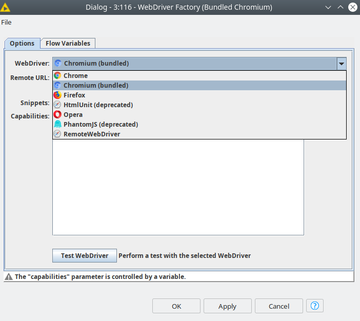
Figure 2. Browser selection in WebDriver Factory node.
Preprocessing Data with Spacy to Do Topic Modeling
Once we have downloaded the subtitles we can read them and extract meta information from the file names – season and episode. There are 5 seasons in Breaking Bad series with different amounts of episodes per season. Topic modeling will be applied for every season independently based on the number of episodes, so we can identify an individual topic for each one. But before applying topic modeling the data should be processed. We are going to use the Redfield NLP Nodes extension that includes Spacy integration. Spacy is a very popular Python-based framework for NLP, that contains a lot of algorithms and language models.
Currently there are 6 Spacy nodes in our extension:
- Spacy Tokenizer – basic operation of splitting the sentences to words and converting them into units called tokens.
- Spacy POS Tagger – assigning the part of speech to the tokens.
- Spacy NER – assigning the named entity tag to the token e.g. location, person name, date, organization, currency, etc.
- Spacy Lemmatizer – converting the token to a root form e.g. singular form, nominative case for noun and adjective and infinitive form for verb.
- Spacy Vectorizer – represent the document as a set of numbers – a vector.
- Spacy Morphologizer – assigning tags for a token form, e.g. gender, singular/plural, case, conjugation, etc.
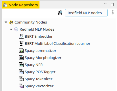
Figure 3. Redfield NLP nodes in the KNIME Node repository.
For data preprocessing we are going to use Tokenizer, POS Tagger, and Lemmatizer nodes. Also, we are going to use Spacy NER node to identify locations, organizations, and person names and then to filter them out so they do not interfere with the topic terms. We are going to use the en_core_web_sm model in all the nodes in the workflow since it has the smallest size and is optimized to run on CPU. First, we need to tokenize the texts – convert individual words in the document to the tokens.
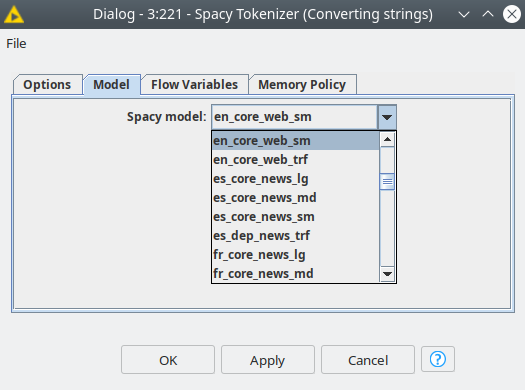
Figure 4. The Spacy model selection dialog.
We developed the nodes this way so that they are compatible with the KNIME Text Processing extension, so after tokenization, we are getting the table with a Document type column. Then we can use KNIME native nodes to clean the texts: Punctuation Erasure – to delete punctuation characters, Case Converter to convert all tokens to lowercase, Stop Word Filter – to clean all non-meaningful words using both in-built and our small customized dictionary. Afterward, we need to make POS tagging using our Spacy POS Tagger. POS tagging is necessary to identify the most meaningful words – we are going to use nouns, verbs, and adjectives. As long as Spacy models might have their own tags, we managed to map Spacy POS tags to the most frequently used POS and UDPOS tag sets. This way we can easily filter the tokens by their tags using the native Tag Filter node.
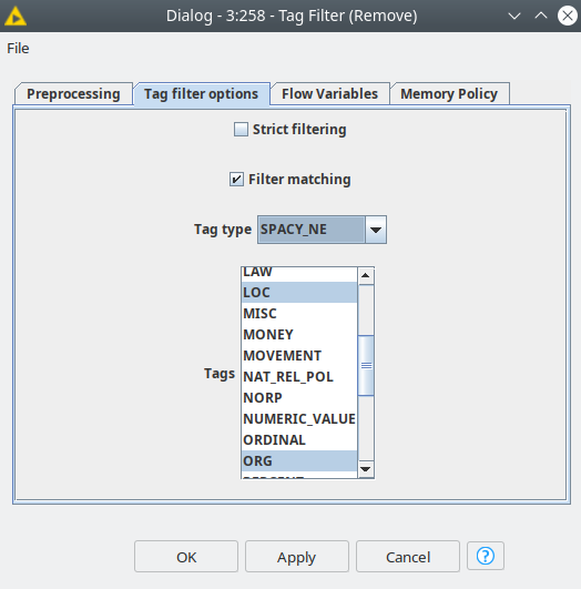
Figure 5. Tag Filter node is compatible with tags assigned by Spacy.
One may ask: KNIME already has a bunch of nodes for text processing and you are actually using some of them, what is the purpose of your extension? The KNIME Text Processing is based on OpenNLP and StanfordNLP frameworks, which unfortunately are not supported anymore. Another problem that the Redfield NLP nodes are solving is the limitation of supported languages. Knime supports seven languages, while Spacy supports 18 languages (and the number is growing): Catalan, Chinese, Danish, Dutch, English, French, German, Greek, Italian, Japanese, Lithuanian, Macedonian, Norwegian Bokmål, Polish, Portuguese, Romanian, Russian, Spanish. Some languages might have more than one model optimized for different types of tasks, also Spacy provides the tools to train your model in case you have a good training data set. Furthermore Spacy is a well-known library in the NLP community and it has good maintenance and it is evolving. This way the combination of the KNIME Text Processing and the Redfield Text Processing gives you more options and flexibility to solve your NLP tasks with KNIME. Let’s say you can use Spacy nodes for pre-processing your data and then refer to Knime’s nodes for topic modeling or term co-occurrence counter. And this is exactly what we are going to do in this example!
Topic Modeling and Clustering
Once the data is processed we can use Group Loop Start and Loop End to iterate over each season, we can grab the number of episodes per season as a flow variable and use it to specify the number of topics in the Topic Extractor (Parallel LDA) node. This way we will try to assign the unique topic to every episode per season.
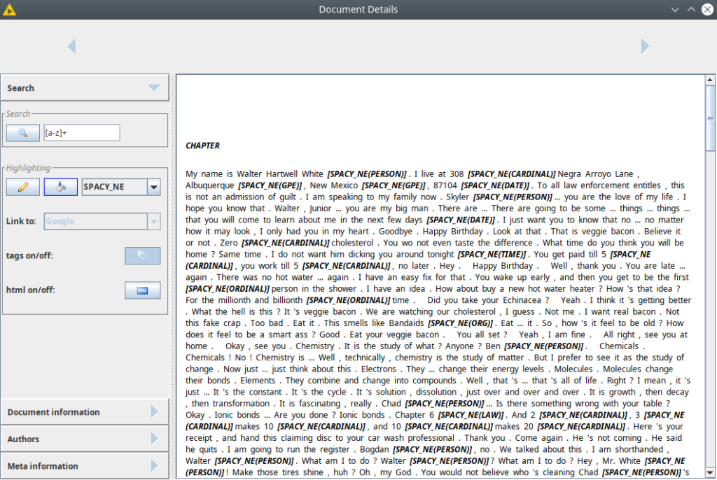
Figure 6. A document with NER tags.
However, usually it does not work and we get the major topic assigned to more than most of the episodes and a couple of minor topics. This is an interesting case that we are going to look at once we plot our results as a knowledge graph of the topic modeling results.
Another approach that we can apply here is to convert the processed texts to vectors and make clustering based on these vectors. Here we need to use the Spacy Vectorizer node. The en_core_web_sm model produces the vector with dimensionality 96. It is fine for algorithms to do clustering, however, it is impossible for a human to do meaningful analysis and make a good plot. So in order to reduce the size of the vector, we are going to apply PCA and t-SNE, so then we can map clustering results to a 3D scatter plot. We are going to set up the number of clusters equal to five – the same as the number of seasons – and use the k-means algorithm. All these algorithms are encapsulated inside the “Clustering and dimensionality reduction” component.

Figure 7. Scatter plots showing clustering results using PCA projections (left) and t-SNE projection (right).
Visualization and Analysis
Once the results of data mining are ready we can visualize the results and analyze them. There are 2 components for visualization that were built for this demo. The first one is called “Clustering analysis” and there we can compare the output of topic modeling and clustering. First, we have the k-means clustering output presented as two projections for PCA and t-SNE. Both projections give similar results – all the clusters are balanced, there are no big distances between samples within one cluster. However one can notice that cluster 1 (red) is the smallest one, at the same time it includes episodes from seasons 3, 4, and 5. And this tendency we can notice for all clusters – they are diverse. This way it is better to compare the distribution of episodes by season vs cluster and assigned topic. This case can be easily visualized with a sunburst diagram. From that diagram we can immediately see that season 3 is the most condensed – most of the episodes are assigned to topic 7 of this season, however, some of the episodes still belong to different clusters, and cluster 0 is the biggest one among them. The most diverse season is season 5 that consists of episodes assigned to five different topics spread among all five clusters. At the same time season, 4 looks a bit strange since episodes are spread along with all five clusters, however, the main topic for all of them is topic 5 of this season. To help to identify all these differences and similarities we are plotting the pivoted table that includes terms of the assigned topics for aggregated by season and topic. And finally, we are plotting the cloud of tags for all the terms based on their weight that we get from LDA.
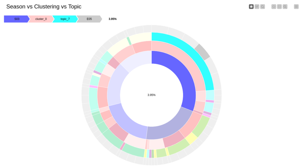
Figure 8. Sunburst diagram showing the distribution of clusters, topics, seasons, and episodes.
Another visualization that we have is a simple knowledge graph that contains information about seasons, episodes, assigned topics, and topic terms. This approach allows us to see the connection between the terms of the topics and the episodes. Furthermore, we can also see which terms are the most frequent since they belong to multiple independent topics. In our case they are mostly the verbs: look, thank, tell, mean, call. At the same time, we clearly see some isolated topics as for episode 8 season 5, episode 2 season 4, episode 13 season 3 where all the terms are unique for just these topics.
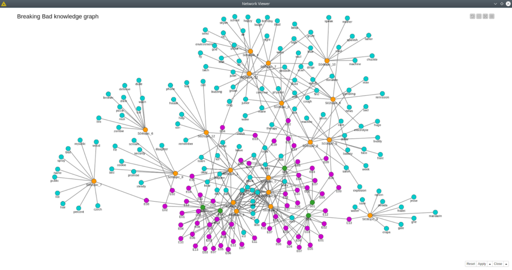
Figure 9. Breaking Bad knowledge graph.
Conclusion
In this demo we managed to solve many problems that businesses face on a daily basis: we scraped the data from an external website, then we processed it, cleaned, and analyzed it with classical NLP algorithms.
Once the data was crunched we applied data mining techniques such as topic modeling, clustering, and dimensionality reduction. Finally, we built two dashboards that made analysis easy and smooth.
Despite having a toy data set in this demo might be easily tweaked to real use case scenarios where one can gather customer reviews of your products or services, or analyze the review of your competitors or understand what is the most discussed in your community.
The Redfield NLP Nodes are now available for free download and 1-month free trial usage. We will be excited to see your workflows solving real NLP problems shared with the community! Share your experience with the nodes.
